Download this page as:

a commented Python script

a minimal Python script

Contents

Frequency Analysis

Frequency Analysis ¶

NumPy is at the core of nearly every scientific Python application or module since it provides a fast N-d array datatype that can be manipulated in a vectorized form. This will be familiar to users of IDL or Matlab.

NumPy has a good and systematic basic tutorial available. It is highly recommended that you read this tutorial to fill in the gaps left by this workshop.

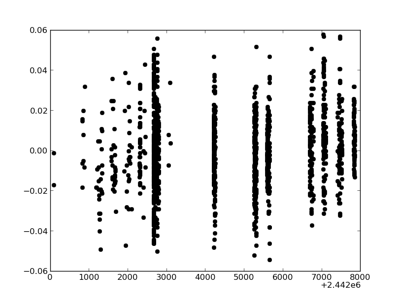
In this tutorial, we are going to take a real observed light curve of the \beta Cephei star HD129929 (after Aerts et al. 2004), and fit a sine through the data:

We assume that the data F_i (i=0,N) can be represented by

F_i = A \sin(\omega t_i + \phi)

We will model the datapoints with a linear least squares. Note that we can write the problem also as

F_i = a \sin(\omega t_i) + b\cos(\omega t_i)

with

A = \sqrt{a^2 + b^2} \phi = \mathrm{arctan} \left(\frac{a}{b}\right)

If we can remove the dependency on the frequency \omega, which is an unknown and nonlinear parameter, the system is linear and we can look for the least-squares solution of the equation

C X = B

That is, the vector X (2x1) that minimizes ||B-CX||^2, with C the Nx2 matrix

C = \left(\begin{array}{cc} \sin(\omega t_1) & \cos(\omega t_1)\\ \sin(\omega t_2) & \cos(\omega t_2)\\ \vdots & \vdots\\ \sin(\omega t_N) & \cos(\omega t_N)\\ \end{array}\right)

and B (Nx1)

B = \left(\begin{array}{c} F_1 \\ \vdots \\ F_N \end{array}\right)

The errors can be estimated as the square root of the diagonal elements of the covariance matrix, once the Jacobian J and sum of squares SS is calculated:

Cov = \frac{SS}{N-2} \left( [J^T J]^{-1} \right)

From a statistical sense, this is not the optimal way of modelling the dataset. It is however, still very useful and traditionally widely applied. One only needs to be careful on how to interpret the results, the derived parameters and their errors.

What’s new ¶

We’ll introduce or further explore:

numpy and scipy: fitting a sine to an observed time series

numpy: creating N-dimensional arrays

numpy: indexing arrays

pyfits: a package for reading and writing FITS files

urllib: a standard library providing common functionality to interface with the internet

Setup ¶

We will use a real FITS-format dataset that we download straight from the ViZieR service. For this, we’ll need the urllib standard library. The dataset is contained in the catalog J/A+A/415/241/table1:

In [1]: import urllib

In [2]: cat = 'J/A+A/415/241/table1'

In [3]: uri = 'http://vizier.u-strasbg.fr/viz-bin/asu-binfits/VizieR?&-source={}&-out.all'.format(cat)

In [4]: url = urllib.URLopener()

In [5]: filen,msg = url.retrieve(uri,filename='cat.fits')

In [6]: url.close()

Reading the data ¶

The FITS-file can easily be read in using pyfits:

In [7]: import pyfits

In [8]: hdus = pyfits.open('cat.fits')

In [9]: hdus
 Out[9]: 
[<pyfits.hdu.image.PrimaryHDU at 0x10e2dd550>,
 <pyfits.hdu.table.BinTableHDU at 0x10e2e3490>]

In [10]: hdus.info()
Filename: cat.fits
No.    Name         Type      Cards   Dimensions   Format
0    PRIMARY     PrimaryHDU      33   ()           uint8
1    J_A_A_415_241_TABLE1  BinTableHDU     60   1493R x 9C   [J, D, E, E, E, E, E, E, E]

Type ?hdus to get a little more detail on the hdus object. Since this FITS file does not contain an image, only the first table extension (second HDU) is important:

In [11]: table = hdus[1].data

Click to Show/Hide Tip: pyFITS

The HDUList from a FITS file acts like an ordered dictionary: instead of accessing via an index n, you can also access the extensions by name:

In [12]: table = hdus['J_A_A_415_241_TABLE1'].data

You can find (and set) the name of an extension throught the header keyword EXTNAME (case-insensitive).

In [13]: hdus[1].header['extname']
Out[13]: 'J_A_A_415_241_TABLE1'

A frequently used convention for images and other telescope data, however, is to store scientific data in an extension named SCI. For more information on FITS files and pyFITS, see the pyFITS documentation

Even if the primary HDU contains no data, the header often contains useful information:

In [14]: hdus[0].header
Out[14]: <pyfits.header.Header at 0x10292fc50>

Let’s have a look at the columns of the data. A lot of information is contained within the header of the table HDU:

In [15]: hdus[1].header
Out[15]: <pyfits.header.Header at 0x10e899c10>

But if you’re only interested in the column names, you can easily retrieve them with

In [16]: hdus[1].columns.names
Out[16]: ['recno', 'HJD', 'Umag', 'B1mag', 'Bmag', 'B2mag', 'V1mag', 'Vmag', 'Gmag']

The two columns we are interested in are the times (HJD) and the visual magnitudes (Vmag). so it is useful to create two new variables for them. Since we don’t need the FITS file anymore, we can close it to free up some memory.

In [17]: hjd = hdus[1].data.field('HJD')

In [18]: vmag = hdus[1].data.field('Vmag')

In [19]: hdus.close()

The variables hjd and vmag are arrays. They have a shape and a type:

In [20]: hjd.shape
Out[20]: (1493,)

In [21]: vmag.dtype
Out[21]: dtype('>f4')

Calculating with arrays ¶

The use of lists in scientific scripting is very limited: they are well suited to store all kinds of information, but they are extremely slow when used in calculations. Numpy arrays are the solution to this problem. They can be easily used in calculations, where one has to remember that all the default operations on array are element-wise:

In [26]: import numpy as np

In [27]: a = np.array([10,20,30,40])

In [28]: b = np.arange(4)

In [29]: a + b**2  # elementwise operation
Out[29]: array([10, 21, 34, 49])

Arrays may have more than one dimension:

In [30]: f = np.ones([3, 4])                 # 3 x 4 float array of ones

In [31]: f
Out[31]: 
array([[ 1.,  1.,  1.,  1.],
       [ 1.,  1.,  1.,  1.],
       [ 1.,  1.,  1.,  1.]])

In [32]: g = np.zeros([2, 3, 4], dtype=int)  # 3 x 4 x 5 int array of zeros

In [33]: i = np.zeros_like(f)                # array of zeros with same shape/type as f

You can change the dimensions of existing arrays:

In [34]: w = np.arange(12)

In [35]: w.shape = [3, 4]       # does not modify the total number of elements

In [36]: w
Out[36]: 
array([[ 0,  1,  2,  3],
       [ 4,  5,  6,  7],
       [ 8,  9, 10, 11]])

In [37]: x = np.arange(5)

In [38]: y = x.reshape(5, 1)

In [39]: y = x.reshape(-1, 1)  # Same thing but NumPy figures out correct length

And you can stack arrays horizontally, vertically, as columns, and make a coordinate grid out of two arrays:

In [40]: x = np.linspace(0,1,3)

In [41]: y = np.linspace(0,10,3)

In [42]: np.hstack([x,y])         # shape (6,)
Out[42]: array([  0. ,   0.5,   1. ,   0. ,   5. ,  10. ])

In [43]: np.vstack([x,y])         # shape (2,3)
Out[43]: 
array([[  0. ,   0.5,   1. ],
       [  0. ,   5. ,  10. ]])

In [44]: np.column_stack([x,y])   # shape (3,2)
Out[44]: 
array([[  0. ,   0. ],
       [  0.5,   5. ],
       [  1. ,  10. ]])

In [45]: xgrid, ygrid = np.meshgrid(x,y)         # 2x shape (3,3)

In [46]: print(xgrid)
[[ 0.   0.5  1. ]
 [ 0.   0.5  1. ]
 [ 0.   0.5  1. ]]

In [47]: print(ygrid)
[[  0.   0.   0.]
 [  5.   5.   5.]
 [ 10.  10.  10.]]

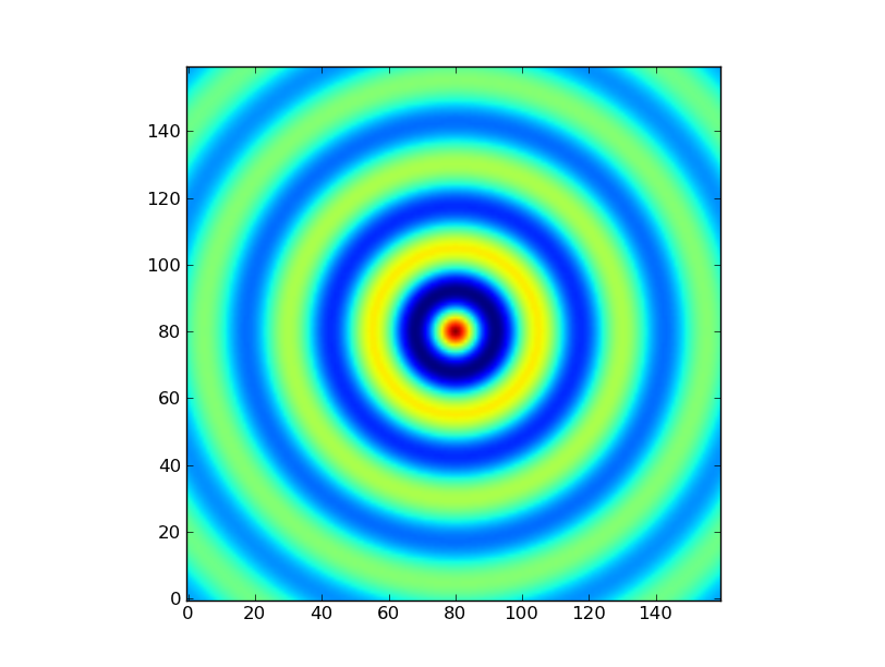
Exercise: Make a ripple

Calculate a surface z = cos(r) / (r + 5) where r = sqrt(x**2 + y**2). Set x and y to an array that goes from -20 to 20 with 160 elements. Use np.meshgrid to generate a coordinate array. Use plt.imshow to display the image of z.

Click to Show/Hide Solution

In [48]: x = np.linspace(-20,20,160)

In [49]: y = np.linspace(-20,20,160)

In [50]: x,y = np.meshgrid(x,y)        # converts x and y into 2D arrays representing coordinates

In [51]: r = np.sqrt(x**2 + y**2)

In [52]: z = np.cos(r) / (r + 5)

In [53]: import matplotlib.pyplot as plt

In [54]: plt.imshow(z)
Out[54]: <matplotlib.image.AxesImage at 0x10e894450>

Finding a frequency ¶

Now we want to compute a frequency spectrum. Since the time series is non-equidistant, we cannot easily use the Fast Fourier Transform implemented in numpy’s FFT pack. Luckily, scipy provides the solution within the scipy.signal package, where a fast implementation of the Lomb-Scargle periodogram is available:

In [55]: import scipy.signal

Let’s search in the frequency interval between 6.2 and 7.2 cy/d, with a frequency resolution equal to one-fifth of the inverse time span (note that lombscargle needs angular frequencies):

In [56]: df = 0.2 / hjd.ptp()

In [57]: freq_interval = np.arange(6.2, 7.2, df)*2*np.pi

Now we can compute the periodogram, after we subtracted the mean from the magnitude array:

In [58]: vmag = vmag - vmag.mean()

In [59]: pgram = scipy.signal.lombscargle(hjd,vmag,freq_interval)
---------------------------------------------------------------------------
ValueError                                Traceback (most recent call last)
/Users/naw/VM-Share/GREAT-ITN/GITN-Meetings/GITN-School-Alicante-Jun13/degroote-doc-v2/<ipython-input-59-53203acdca39> in <module>()
----> 1 pgram = scipy.signal.lombscargle(hjd,vmag,freq_interval)

/Library/Frameworks/EPD64.framework/Versions/7.3/lib/python2.7/site-packages/scipy/signal/spectral.so in scipy.signal.spectral.lombscargle (scipy/signal/spectral.c:1119)()

ValueError: Big-endian buffer not supported on little-endian compiler

Oops! What happened here? Apparently, the Lomb-Scargle periodogram fails to compute, and it has something to do with the type of the array. The Lomb-Scargle function is picky about the dtype of the array it receives. Since we loaded the times and magnitudes from a FITS record, these arrays (can) have a non-standard data type. Although this looks more like an omission in the Lomb-Scargle function (it should check for this and cast arrays to the right format), this is easily fixed by converting them to normal float arrays manually:

In [60]: hjd = np.array(hjd,float)

In [61]: vmag = np.array(vmag,float)

In [62]: pgram = scipy.signal.lombscargle(hjd,vmag,freq_interval)

Exercise: Normalise the periodogram

The periodogram from scipy’s lombscargle is a power spectrum, not an amplitude spectrum. Look at the documentation to figure out how to normalise it to an amplitude spectrum. Perform the normalisation and make a plot of the amplitude spectrum versus cyclical frequency, using a black connected line.

Click to Show/Hide Solution

In [63]: Ndata = len(hjd)         # equivalent to Ndata = hjd.shape[0]

In [64]: norm = np.sqrt(4.0 * pgram / Ndata)

In [65]: freq_interval_cy = freq_interval/(2*np.pi)

In [66]: plt.plot(freq_interval_cy,norm,'k-')
Out[66]: [<matplotlib.lines.Line2D at 0x10f29fc50>]

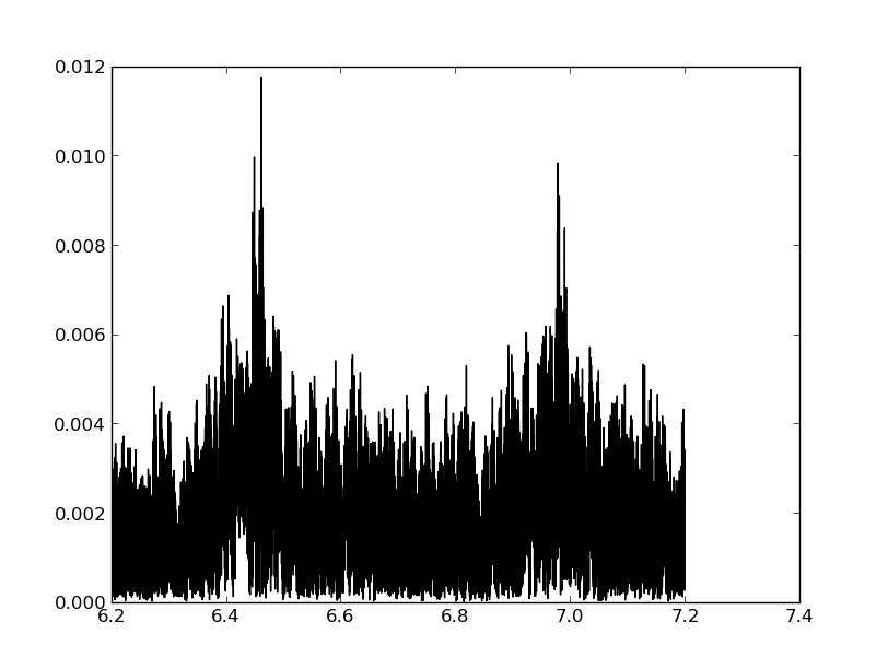
The frequency that is most likely present in the data is the one that has the highest peak in the periodogram. We can easily retrieve it via:

In [67]: freq = freq_interval[np.argmax(pgram)]

In [68]: print(freq/(2*np.pi))
6.46169456447

The function argmax returns the index of the maximum value. We use that index to recover the frequency at that index. The value from the paper is 6.461699 cy/d.

Fitting a sine ¶

Now let us create the array C as described in the introduction and call the least square solver lstsq from the linear algebra module:

In [69]: C = np.column_stack([np.sin(freq*hjd), np.cos(freq*hjd)])

In [70]: X, sumsq, rank, s = np.linalg.lstsq(C,vmag)

Now retrieve the value for the amplitude and the phase (see introduction):

In [71]: amplitude = np.sqrt(X[0]**2 + X[1]**2)

In [72]: phase = np.arctan2(X[1],X[0])

In [73]: fit = amplitude * np.sin(freq*hjd + phase)

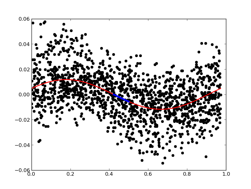
A phasediagram can be a good way of evaluating the fit by eye. The phases are easily calculated and plotted with:

In [74]: phased = 2*np.pi * (hjd % (2*np.pi/freq))      # frequency in rad/s, but time in s!

In [75]: plt.plot(phased,vmag,'ko');

The fit, however, we want to plot as a connected line. To do this, we need to sort the phases, as the order of the phases is still chronological:

In [76]: hjd
Out[76]: 
array([ 2442095.88 ,  2442096.88 ,  2442829.873, ...,  2449853.744,
        2449853.758,  2449853.779])

In [77]: phased
Out[77]: 
array([ 0.65509455,  0.13166021,  0.4981324 , ...,  0.6041817 ,
        0.69214629,  0.82409318])

Indexing ¶

We’ve seen above that we can easily select an element from an array, and even ranges with strides. Indexing can also be done with integer arrays and boolean arrays. It is easiest to understand integer indexing when seen in action:

In [78]: x = np.linspace(0,1,11)

In [79]: print(x)
[ 0.   0.1  0.2  0.3  0.4  0.5  0.6  0.7  0.8  0.9  1. ]

In [80]: index = np.array([0,1,2,3,4])

In [81]: print(x[index])
[ 0.   0.1  0.2  0.3  0.4]

In [82]: index = np.array([0,3,1,4,2])

In [83]: print(x[index])
[ 0.   0.3  0.1  0.4  0.2]

You can use this to sort one array with another array via numpy’s argsort:

In [84]: x = np.random.uniform(size=5)

In [85]: x
Out[85]: array([ 0.78447263,  0.48100051,  0.84391752,  0.66880414,  0.67966193])

In [86]: index = np.argsort(x)

In [87]: index
Out[87]: array([1, 3, 4, 0, 2])

In [88]: x[index]
Out[88]: array([ 0.48100051,  0.66880414,  0.67966193,  0.78447263,  0.84391752])

Alternatively, it is possible to index arrays with boolean arrays, allowing conditional selection. Again, seeing it in action clarifies things:

In [89]: x = np.linspace(0,1,11)

In [90]: x
Out[90]: array([ 0. ,  0.1,  0.2,  0.3,  0.4,  0.5,  0.6,  0.7,  0.8,  0.9,  1. ])

In [91]: index = np.array([True,False,True,True])

In [92]: x[index]
Out[92]: array([ 0. ,  0.2,  0.3])

You can use this for example to select all positive numbers from an array:

In [93]: x = np.random.normal(size=5)

In [94]: x
Out[94]: array([ 0.03195249, -1.06447481, -2.03012963,  0.61535761, -0.46198094])

In [95]: is_positive = x > 0

In [96]: is_positive
Out[96]: array([ True, False, False,  True, False], dtype=bool)

In [97]: x[is_positive]
Out[97]: array([ 0.03195249,  0.61535761])

You can combine conditions element-wise with the operators & (and) and | (or). We can use both methods to plot the fit as a thick connected red line, and the negative values in the first half of the phase as a (very) thick blue line:

In [98]: sortarray = np.argsort(phased)

In [99]: select = (fit[sortarray] < 0) & (phased[sortarray] < 0.5)

In [100]: plt.plot(phased[sortarray], fit[sortarray], 'r-',lw=2);

In [101]: plt.plot(phased[sortarray][select], fit[sortarray][select], 'b-',lw=4);

Calculating errors ¶

To compute the errors, we first need to compute the Jacobian, which contains the partial derivatives of the fitting function:

In [102]: J = np.column_stack([np.sin(freq*hjd + phase), amplitude * np.cos(freq*hjd + phase)])

In [103]: cov = sumsq / (Ndata - 2) * np.linalg.inv(np.dot(J.T, J))

In [104]: e_amplitude = np.sqrt(cov.diagonal()[0])

In [105]: e_phase = np.sqrt(cov.diagonal()[1])

In [106]: print("Amplitude = {:.4f} +/- {:.4f} mag".format(amplitude,e_amplitude))
Amplitude = 0.0118 +/- 0.0006 mag

In [107]: print("Phase = {:.2f} +/- {:.2f} rad".format(phase,e_phase))
Phase = 0.41 +/- 0.05 rad

Wrapping up ¶

An uninterrupted version of what we’ve done:

import numpy as np
import matplotlib.pyplot as plt
import scipy.signal
import urllib
import pyfits

# Download data
cat = 'J/A+A/415/241/table1'
uri = 'http://vizier.u-strasbg.fr/viz-bin/asu-binfits/VizieR?&-oc=deg,eq=J2000&-source={}&-out.all'.format(cat)
url = urllib.URLopener()
filen,msg = url.retrieve(uri,filename='cat.fits')
url.close()

# Read the FITS file
with pyfits.open('cat.fits'):
    hdus = pyfits.open('cat.fits')
    hjd = np.array(hdus[1].data.field('HJD'),float)
    vmag = np.array(hdus[1].data.field('Vmag'),float)

# Subtract mean from data
vmag = vmag - vmag.mean()

# Compute the periodogram and retrieve the frequency
df = 0.2 / hjd.ptp()
freq_interval = np.arange(6.2, 7.2, df)*2*np.pi
pgram = scipy.signal.lombscargle(hjd,vmag,freq_interval)
freq = freq_interval[np.argmax(pgram)]

# Perform the linear fit
C = np.column_stack([np.sin(freq*hjd), np.cos(freq*hjd)])
X, sumsq, rank, s = np.linalg.lstsq(C,vmag)

# Retrieve the parameters
amplitude = np.sqrt(X[0]**2 + X[1]**2)
phase = np.arctan2(X[1],X[0])
fit = amplitude * np.sin(freq*hjd + phase)

# Compute the errors
Ndata = len(hjd)
J = np.column_stack([np.sin(freq*hjd + phase), amplitude * np.cos(freq*hjd + phase)])
cov = sumsq / (Ndata - 2) * np.linalg.inv(np.dot(J.T, J))
e_amplitude = np.sqrt(cov.diagonal()[0])
e_phase = np.sqrt(cov.diagonal()[1])

# Report results
print("Frequency = {:.6f} cy/d".format(freq/(2*np.pi)))
print("Amplitude = {:.4f} +/- {:.4f} mag".format(amplitude,e_amplitude))
print("Phase = {:.2f} +/- {:.2f} rad".format(phase,e_phase))

Note the use of the with statement instead of the open / close paradigm.

Summary ¶

Array properties

Access via:

myarray.<PROPERTY>

`dtype`_	Data-type of the array’s elements.
shape	Tuple of array dimensions.

Basic statistics

Some of the functions below have duplicate definitions as array properties. This is somewhat confusing, so it is advised to always use:

mymean = np.mean(myarray)

instead of:

mymean = myarray.mean()

All array methods have function equivalents, but not vice versa.

np.mean()	Compute the arithmetic mean along the specified axis.
np.average()	Compute the weighted average along the specified axis.
np.median()	Compute the median along the specified axis.
np.std()	Compute the standard deviation along the specified axis.
np.ptp()	Range of values (maximum - minimum) along an axis.
np.max()	Return the maximum of an array or maximum along an axis.
np.min()	Return the minimum of an array or minimum along an axis.
np.argmax()	Indices of the maximum values along an axis.
np.argmin()	Indices of the minimum values along an axis.

Creating arrays

np.array()	Create an array
np.linspace()	Return evenly spaced numbers over a specified interval.
np.arange()	Return evenly spaced values within a given interval.
np.logspace()	Return numbers spaced evenly on a log scale.
np.meshgrid()	Return coordinate matrices from two or more coordinate vectors.
np.zeros()	Return a new array of given shape and type, filled with zeros.
np.zeros_like()	Return an array of zeros with the same shape and type as a given array.
np.ones()	Return a new array of given shape and type, filled with ones.
np.ones_like()	Return an array of ones with the same shape and type as a given array.
np.reshape()	Gives a new shape to an array without changing its data.

Combining arrays

np.hstack()	Stack arrays in sequence horizontally (column wise).
np.vstack()	Stack arrays in sequence vertically (row wise).
np.column_stack()	Stack 1-D arrays as columns into a 2-D array.
np.dstack()	Stack arrays in sequence depth wise (along third axis).

Table Of Contents

Previous topic

Next topic

This Page