A worked out example: determining nu_max

In this example, we use numpy to determine the \nu_\mathrm{max} of a red giant. We’ll read and plot the power spectrum, smooth it using convolution, and fit a non-linear model to the smoothed spectrum.

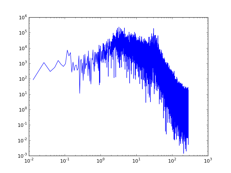
• First we read the power spectrum from a file. By now, you already know how to read a dataset from an ascii file:

  >>> import numpy as np
  >>> data = np.loadtxt("ps5900096_B.txt")
  >>> freq = data[:,0]
  >>> spectrum = data[:,1]
  >>> plt.loglog(freq, spectrum)
  

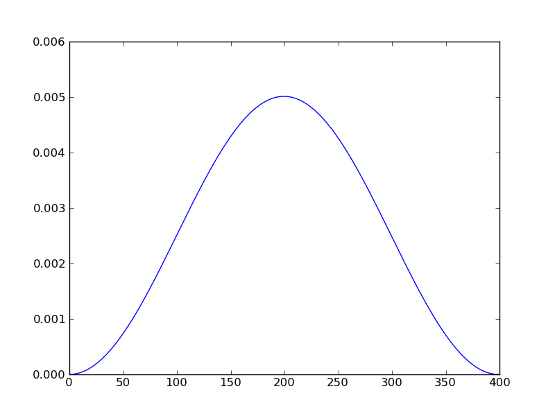
• We would like to smooth the spectrum by convolving with a (normalized) Hann window of 400 points

  >>> kernel = np.hanning(400)
  >>> kernel = kernel / kernel.sum()
  >>> plt.plot(kernel)
  

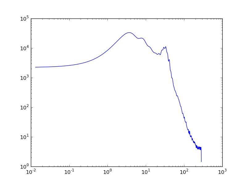
• The smoothing can simply be done with a convolution. The numpy convolve() method has 3 different modes, depending whether you accept boundary effects where the convolution is not perfect because your dataset is finite. ‘FULL’ leads to a convolved array with a size larger than the original, because it returns all the points where there is overlap between the spectrum and the kernel. ‘SAME’ keeps the size of the convolved array the same as the one of the original array; boundary effects can be seen. ‘VALID’ leads to a smaller convolved array than the original, because it only returns the point where there is complete overlap so that no boundary effects are seen. For this exercise we don’t care much about boundary effects, so we use ‘SAME’ which has the convenience that the array size doesn’t change.

  >>> smoothed = np.convolve(kernel, spectrum, mode='SAME')
  >>> plt.loglog(freq, smoothed)
  

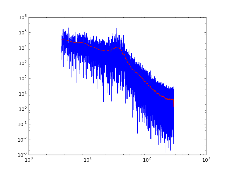
• The low-frequency part of the spectrum is not physical but comes from the instrumental detrending. We therefore crop the spectrum to remove that part.

  >>> spectrum = spectrum[freq >= 3.6]
  >>> smoothed = smoothed[freq >= 3.6]
  >>> freq = freq[freq >= 3.6]
  >>> plt.loglog(freq, spectrum)
  >>> plt.loglog(freq, smoothed, c='r')
  

• Next, we’ld like to fit the smoothed spectrum. Our model is a background (due to granulation), a gaussian to characterize the power excess due to oscillations, and a constant white noise due to photon noise. First our fit function:

  >>> def fitfunc(freq, x):
  ...     # x = fit parameters
  ...     fit = x[0] / (1 + (x[1] * (freq-x[2]))**2) +  + x[3] * np.exp(-(freq-x[4])**2/2.0/x[5]**2) + x[6]
  ...     return fit
  

  Then the chi-square that we would like to minimize:

  >>> def chisquare(fitparam, freq, spectrum):
  ...     fit = fitfunc(freq, fitparam)
  ...     chisq = np.sum((spectrum - fit)**2)
  ...     return chisq
  

  The routine we use to minimize is the build-in optimizer that uses the Powell algorithm:

  >>> from scipy.optimize import fmin_powell
  

  which needs an initial guess of the parameters before it can start:

  >>> initialGuess = np.array([1.e4, 0.01, 4.0, 2.e4, 0.1, 0.03, 1.0, 30.0, 10.0, 10.0])
  >>> bestFitParam = fmin_powell(chisquare, initialGuess, args=(freq, smoothed))
  

  Be aware that non-linear fitting is an art, not a science!

• We plot our results:

  >>> bestFit = fitfunc(freq, bestFitParam)
  >>> plt.plot(freq, smoothed)
  >>> plt.plot(freq, bestFit, c='r')
  >>> plt.xlim(0.0, 100.)
  

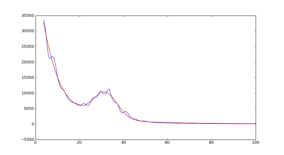
• That’s it! The parameter we were after is \nu_\mathrm{max}:

  >>> nuMax = bestFitParam[7]
  >>> nuMax
  31.6834631635