Bayesian parameter estimation and model comparison

For the example scripts below to run, you will need to import the following modules:

import numpy as np
from numpy import sum
import matplotlib.pyplot as plt
from scipy.stats import distributions

Is this coin fair?

Uniform prior

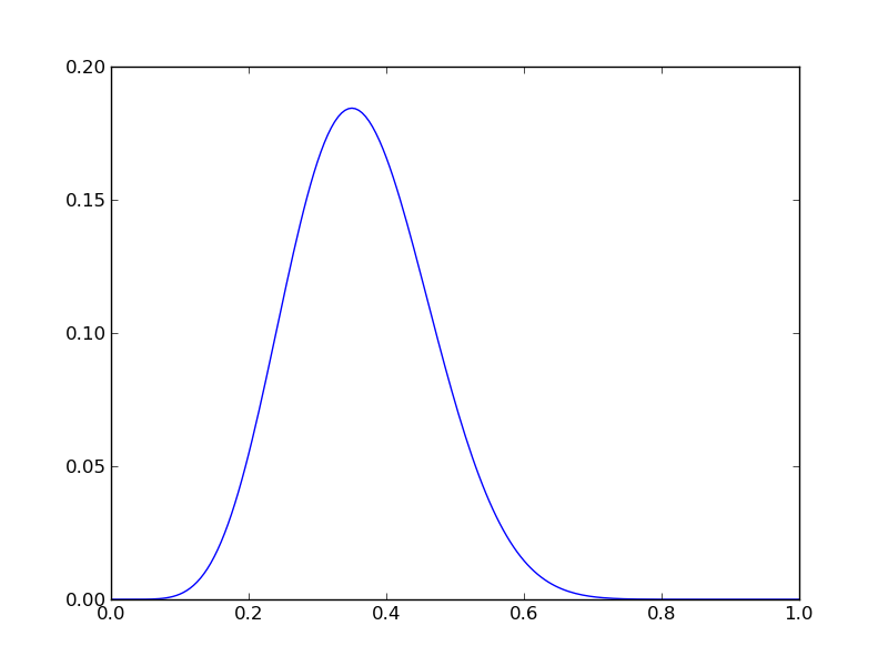
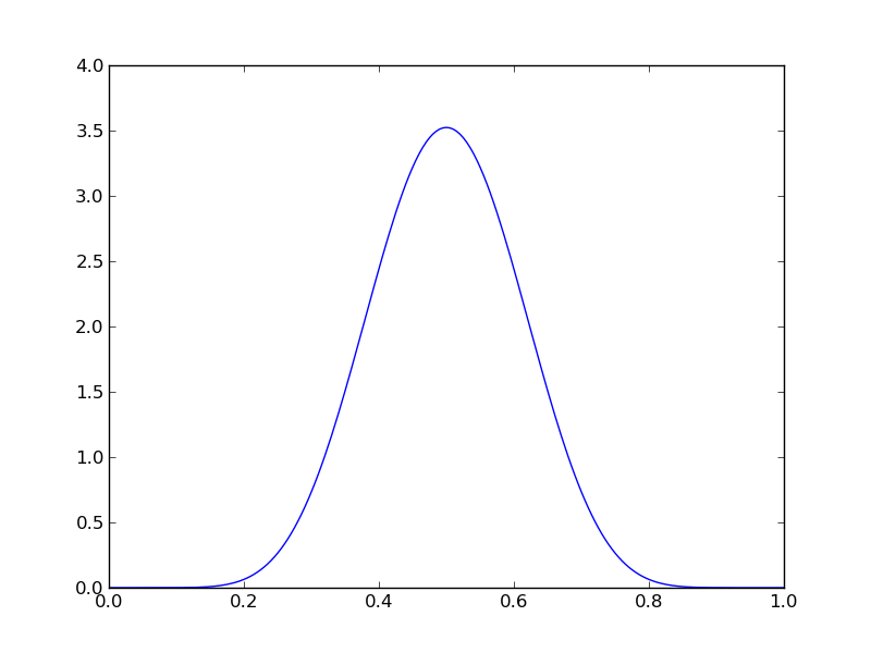
Imagine we had n=20, r=7. We can plot the posterior PDF using

n = 20
r = 7
Nsamp = 201 # no of points to sample at
p = np.linspace(0,1,Nsamp)
pdense = distributions.binom.pmf(r,n,p) # probability mass function
plt.plot(p,pdense)
plt.savefig('fig01.png')

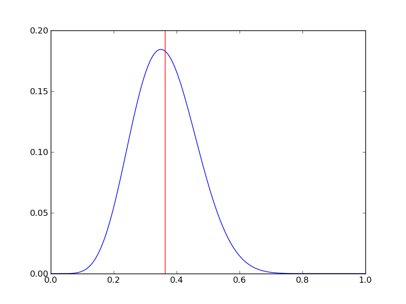
Implementing this in Python and plotting

pdense = distributions.binom.pmf(r,n,p) # probability mass function
p_mean = sum(p*pdense)/sum(pdense)
plt.axvline(p_mean,color='r')
plt.savefig('fig02.png')
plt.close()

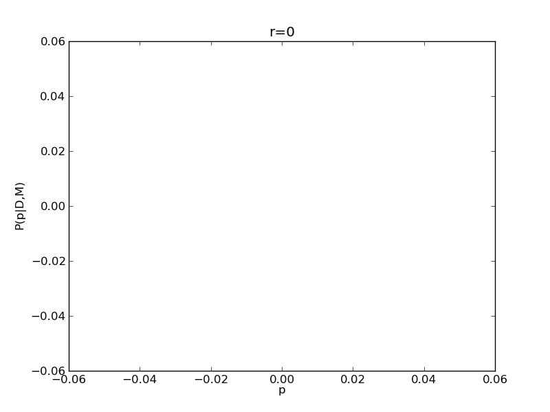
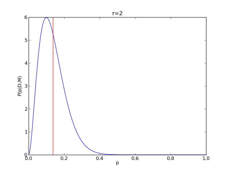
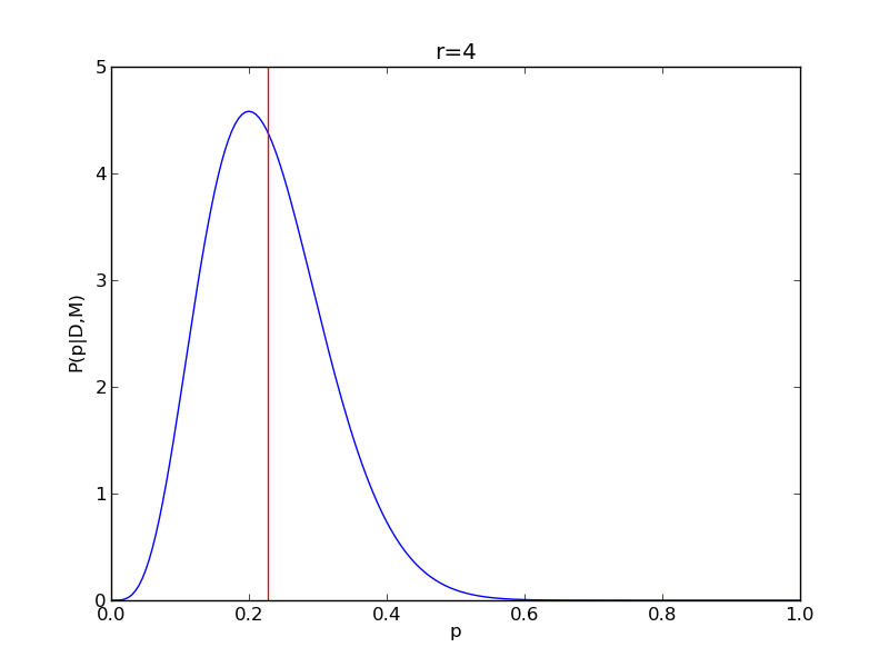
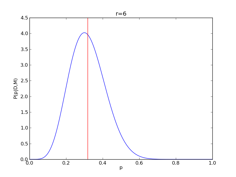
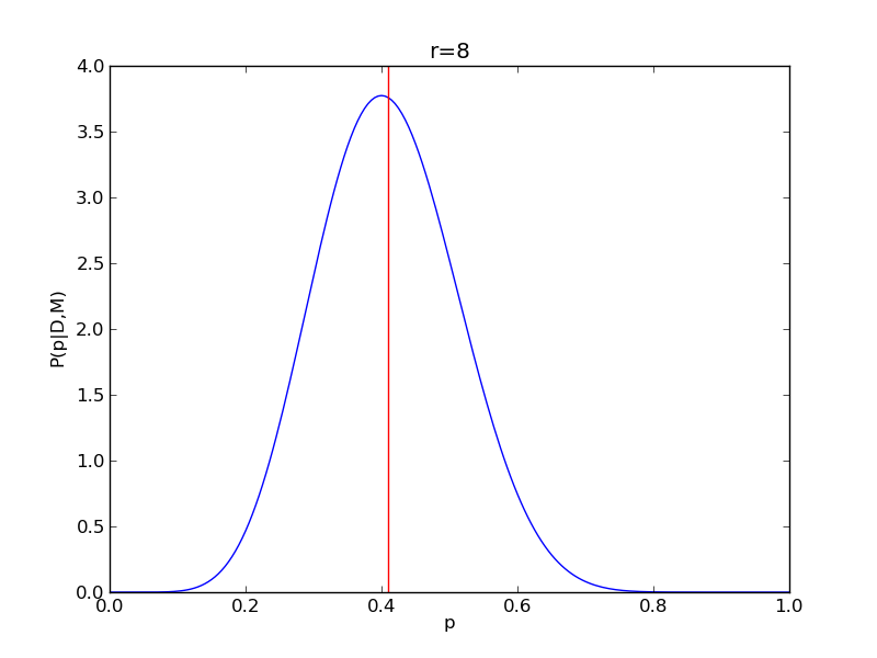
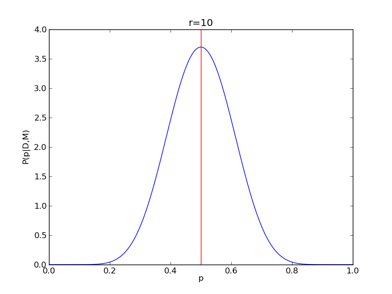
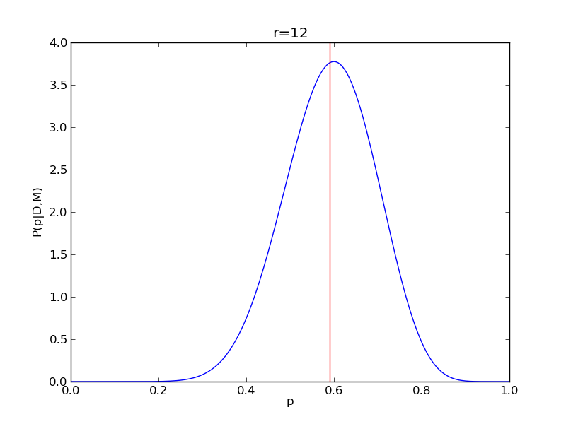
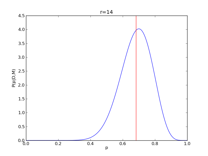
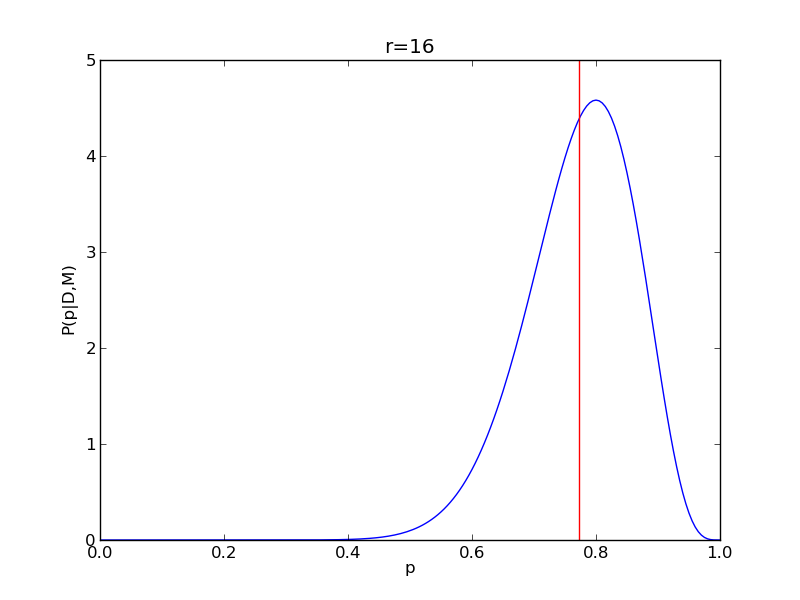
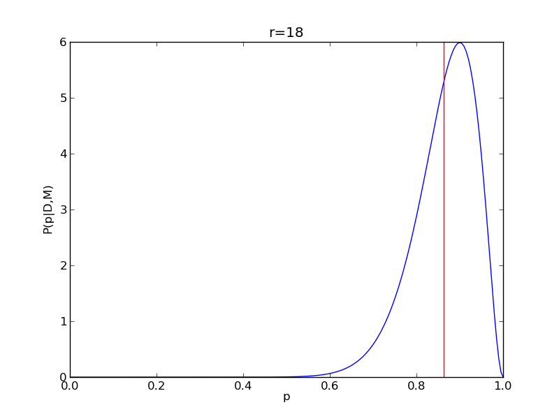
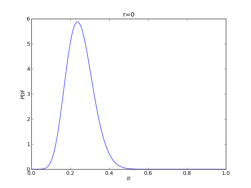
It is instructive to repeat this example for n=20 for a range of values of r.

n = 20
Nsamp = 201
p = np.linspace(0,1,Nsamp)
deltap = 1./(Nsamp-1) # step size between samples of p

for r in range(0,20,2):

    # compute posterior
    pdense = distributions.binom.pmf(r,n,p)
    pdense = pdense / (deltap*sum(pdense)) # normalize posterior
    # compute mean
    p_mean = sum(p*pdense)/sum(pdense)

    # make the figure
    plt.figure()
    plt.plot(p,pdense)
    plt.axvline(p_mean,color='r')
    plt.xlabel('p')
    plt.ylabel('P(p|D,M)')
    plt.title('r={}'.format(r))
    plt.savefig('fig03_r{}'.format(r))
    plt.close()

Beta prior

Let’s now redo the coin analysis with a beta prior with \alpha=\beta=10

alpha = 10
beta = 10
Nsamp = 201 # no of points to sample at

p = np.linspace(0,1,Nsamp)
pdense = distributions.beta.pdf(p,alpha,beta) # probability mass function

plt.plot(p,pdense)
plt.savefig('fig04.png')

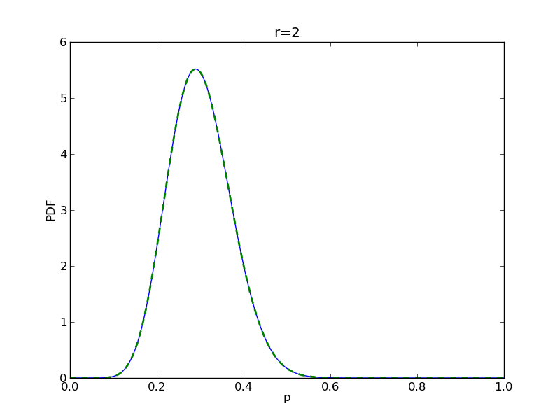
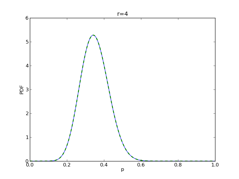
alpha = 10
beta = 10
n = 20
Nsamp = 201 # no of points to sample at


deltap = 1./(Nsamp-1) # step size between samples of p
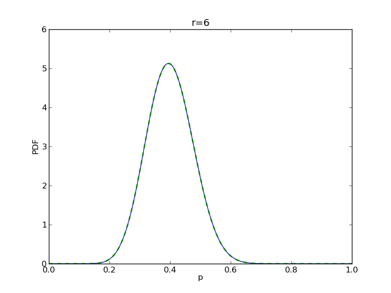
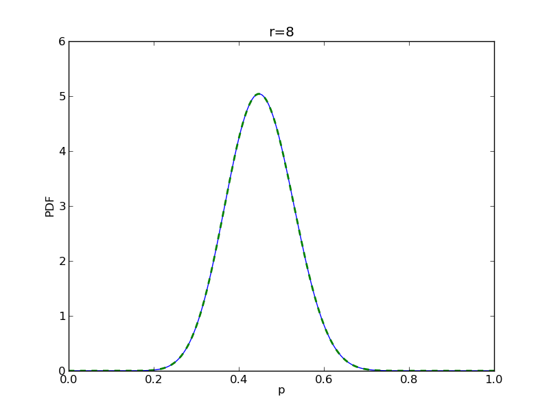
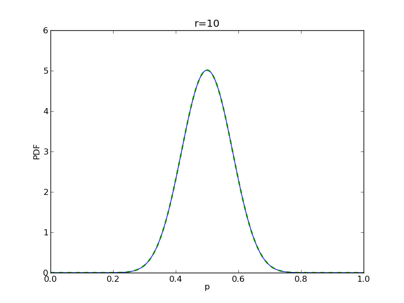
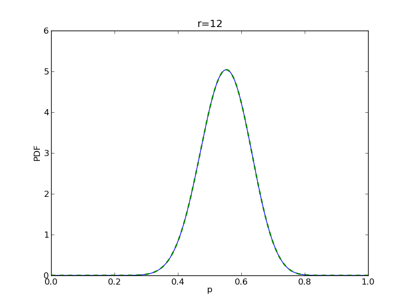
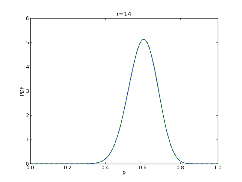
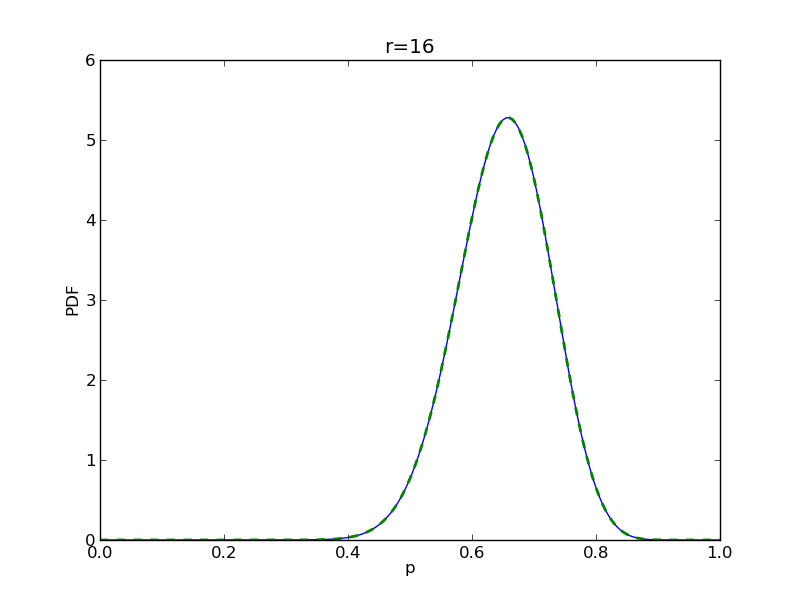
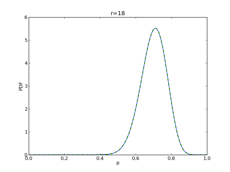
for r in range(0,20,2):

    # compute posterior
    pdense = distributions.beta.pdf(p,alpha+r,beta+n-r)
    pdense2 = distributions.binom.pmf(r,n,p) * distributions.beta.pdf(p,alpha,beta)
    pdense2 = pdense2 / (deltap*sum(pdense2)) # normalize posterior

    # make the figure
    plt.figure()
    plt.plot(p,pdense)
    plt.plot(p,pdense2,'--',lw=2)
    plt.xlabel('p')
    plt.ylabel('PDF')
    plt.title('r={}'.format(r))
    plt.savefig('fig05_r{}'.format(r))

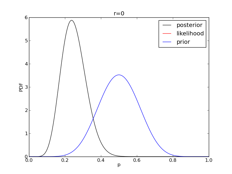
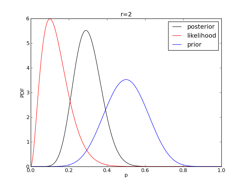
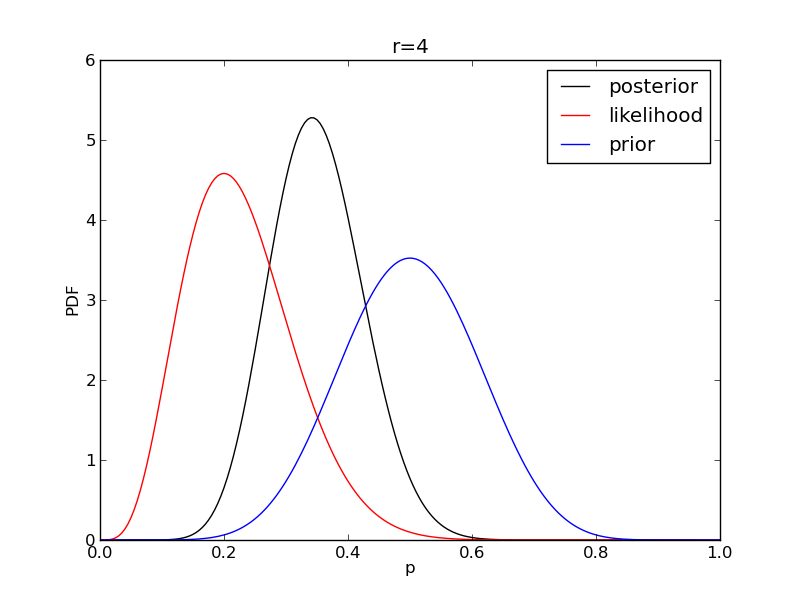
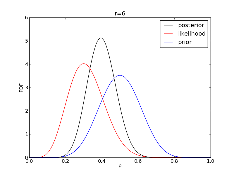
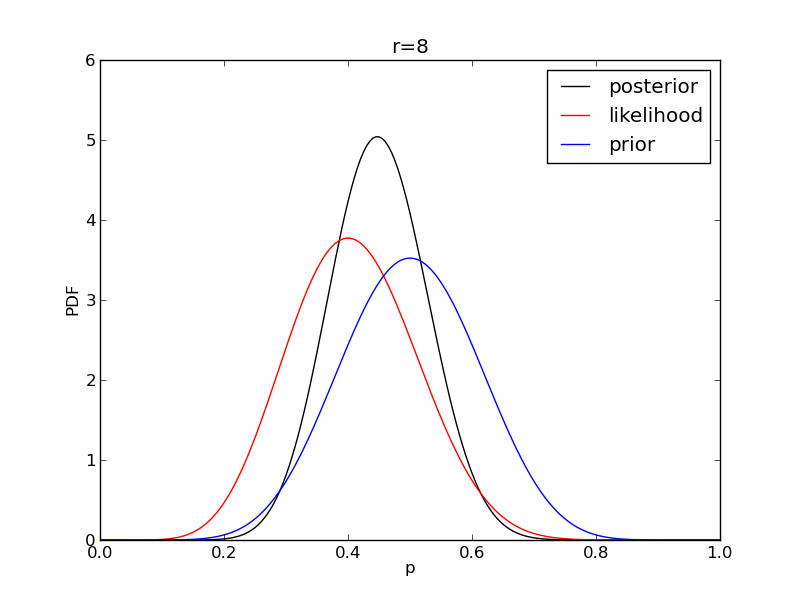
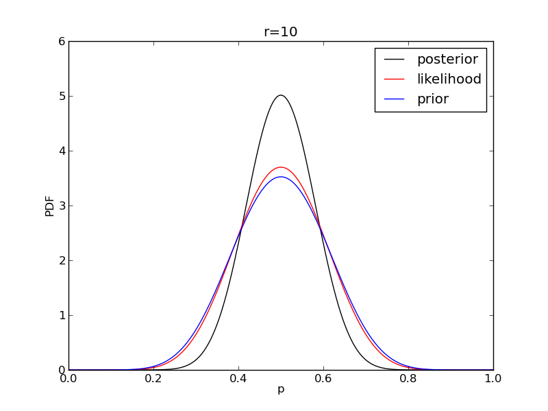
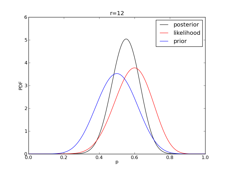
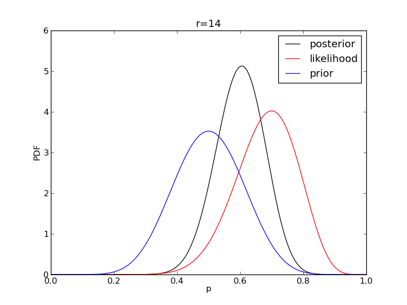
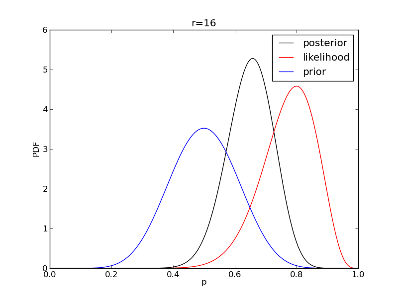
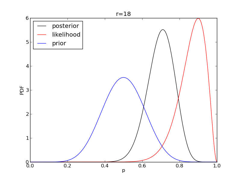
It is instructive to plot the likelihood, prior and posterior together:

alpha = 10
beta = 10
n = 20
Nsamp = 201 # no of points to sample at
deltap = 1./(Nsamp-1) # step size between samples of p

prior = distributions.beta.pdf(p,alpha,beta)

for r in range(0,20,2):

    like = distributions.binom.pmf(r,n,p)
    like = like/(deltap*sum(like)) # for plotting convenience only: see below
    post = distributions.beta.pdf(p,alpha+r,beta+n-r)

    # make the figure
    plt.figure()
    plt.plot(p,post,'k',label='posterior')
    plt.plot(p,like,'r',label='likelihood')
    plt.plot(p,prior,'b',label='prior')
    plt.xlabel('p')
    plt.ylabel('PDF')
    plt.legend(loc='best')
    plt.title('r={}'.format(r))
    plt.savefig('fig06_r{}'.format(r))

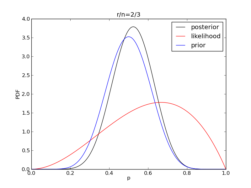
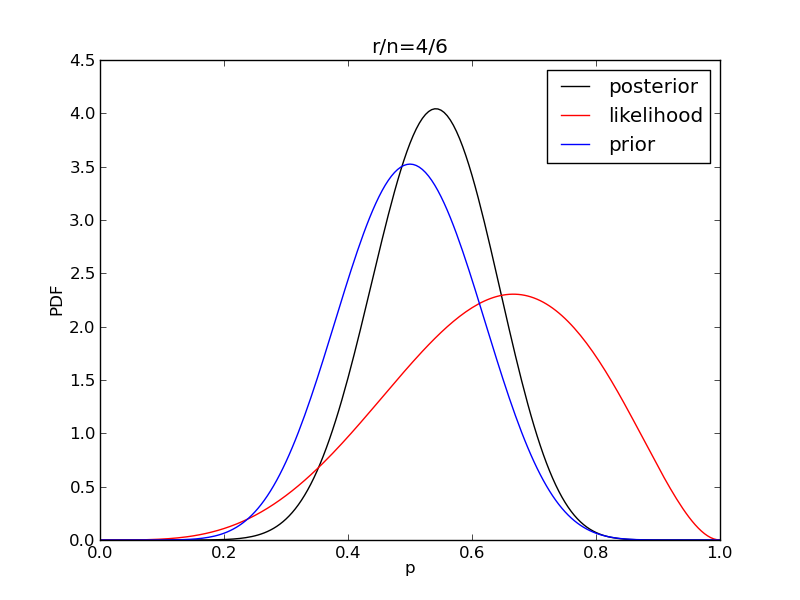
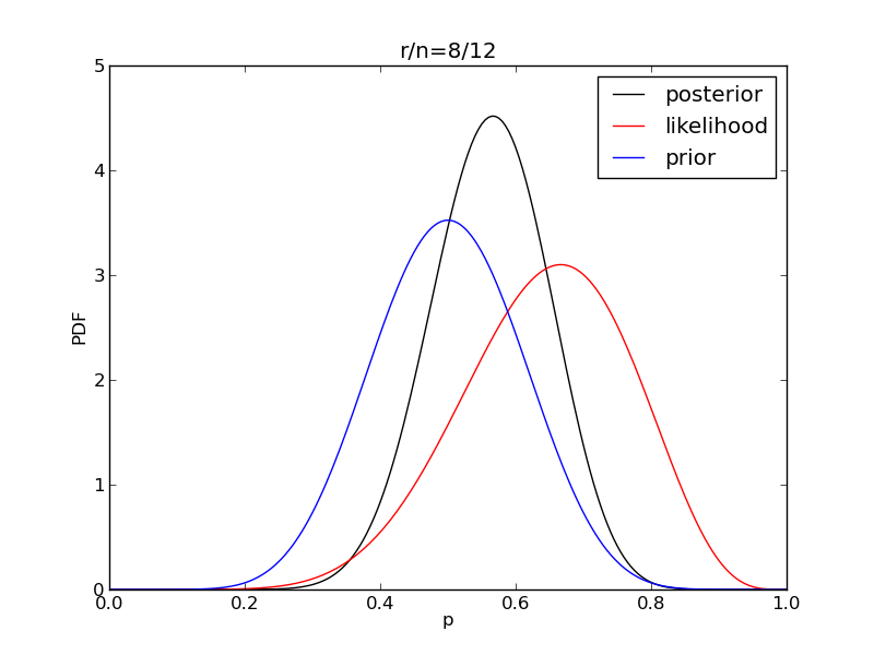
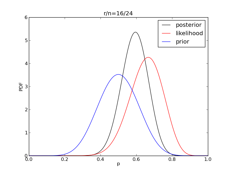
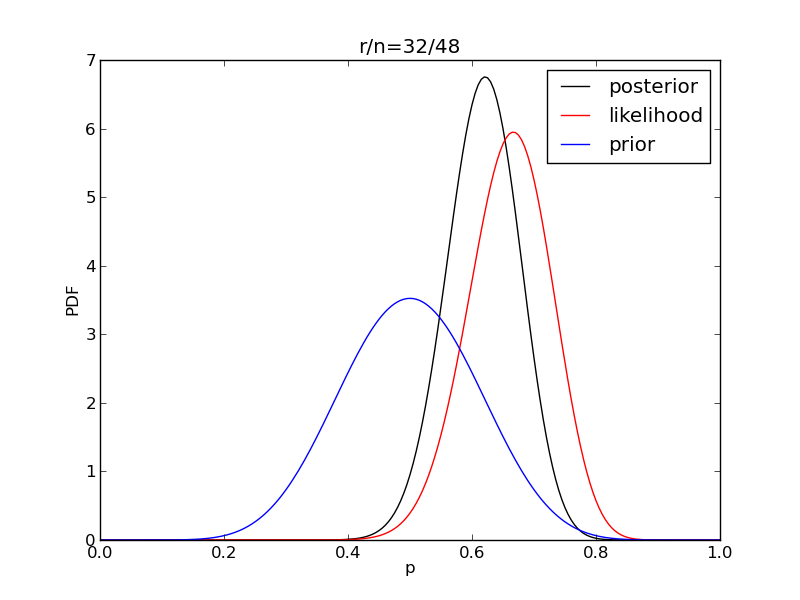
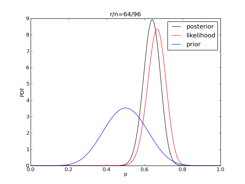
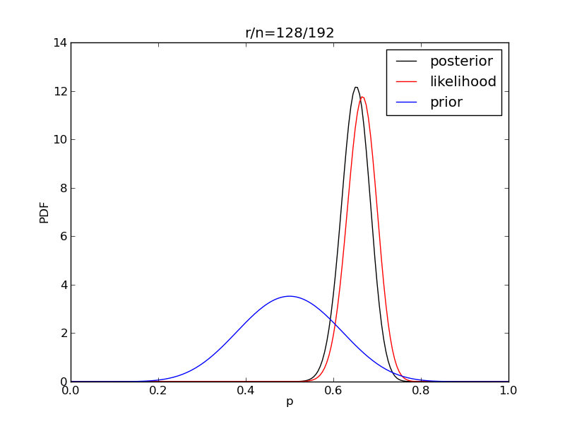
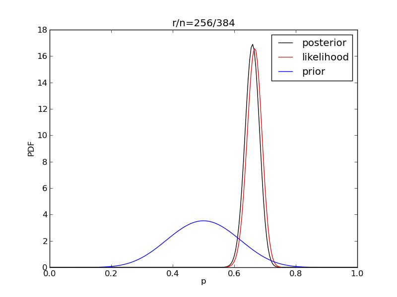
It is interesting to see how the likelihood and posterior evolve as we get more data.

alpha = 10
beta = 10
n = 20
Nsamp = 201 # no of points to sample at
deltap = 1./(Nsamp-1) # step size between samples of p

prior = distributions.beta.pdf(p,alpha,beta)

for i in range(1,9):

    r = 2**i
    n = (3.0/2.0)*r
    like = distributions.binom.pmf(r,n,p)
    like = like/(deltap*sum(like)) # for plotting convenience only
    post = distributions.beta.pdf(p,alpha+r,beta+n-r)

    # make the figure
    plt.figure()
    plt.plot(p,post,'k',label='posterior')
    plt.plot(p,like,'r',label='likelihood')
    plt.plot(p,prior,'b',label='prior')
    plt.xlabel('p')
    plt.ylabel('PDF')
    plt.legend(loc='best')
    plt.title('r/n={}/{:.0f}'.format(r,n))
    plt.savefig('fig07_r{}'.format(r))