The package scipy.stats
The scipy.stats module specializes in random variables and probability distributions. It implements more than 80 continuous distributions and 10 discrete distributions. In what follows we learn how to use the basic functionality. For the more detailed reference manual we refer to http://docs.scipy.org/doc/scipy/reference/stats.html.
Contents
Probability distributions
First import the modules:
>>> import numpy as np
>>> from scipy import stats
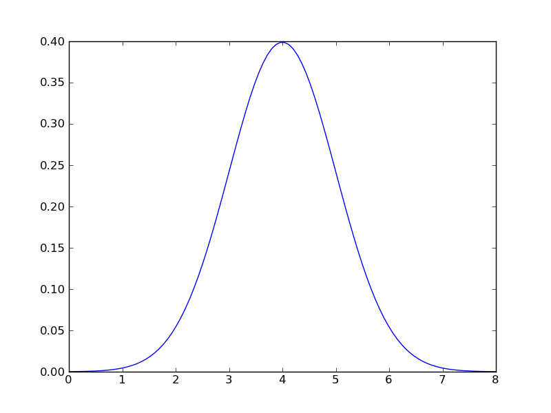
In what follows we will use a gaussian distribution with mean = 2.0, and a standard deviation of 1.0:
>>> gaussian = stats.norm(loc=4.0, scale=1.0)
It’s easy to plot the probability distribution:
>>> x = np.linspace(0.0, 8.0, 100)
>>> y = gaussian.pdf(x)
>>> plt.plot(x,y)
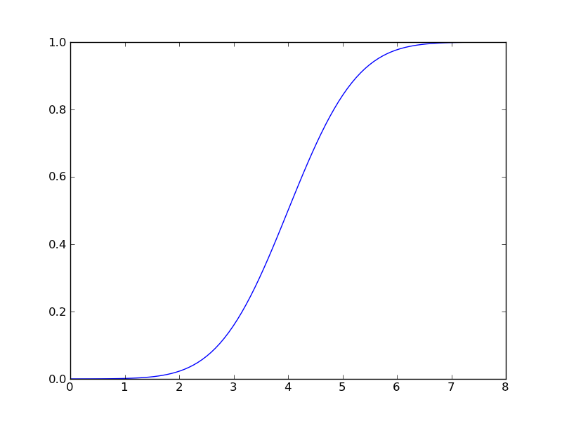
Or the cumulative distribution:
>>> z = gaussian.cdf(x)
>>> plt.plot(x,z)
The module provides an easy-to-use way to compute the mean (‘m’), the variance (‘v’), the skewness (‘s’) and the kurtosis (‘k’):
>>> gaussian.stats(moments="mvsk")
(array(4.0), array(1.0), array(0.0), array(0.0))
As expected, the gaussian distribution has zero skewness and zero kurtosis.
For hypothesis testing, one often needs the p-value. For example, for the given gaussian distribution above, what would be the x-value so that P(X <= x) = 0.95?
>>> gaussian.ppf(0.95)
5.6448536269514724
Drawing 1000 random values is straightforward:
>>> x = gaussian.rvs(1000)
>>> plt.hist(x, bins=40, normed=True)
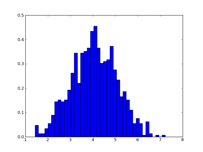
What about the other way around? Given the sample ‘x’, can we fit a gaussian distribution and retrieve the mean and the variance again?
>>> location, scale = stats.norm.fit_loc_scale(x)
>>> print(location, scale)
(4.0274461188878572, 1.024240213225319)
Of course, we can fit any distribution to our sample:
>>> location, scale = stats.logistic.fit_loc_scale(x)
>>> print(location, scale)
(4.0274461188878572, 0.56469322540409594)
Testing the distribution
Suppose you have a sample of data, and you’ld like to find out whether it’s consistent with a, say, Student’s-t distribution. How can scipy.stats help you?
Let’s first make some artificial data:
>>> dof = 10    # degrees of freedom
>>> x = stats.t.rvs(dof, size = 1000)
and let’s pretend we are not sure the sample is drawn from a standard t-distribution.
First, there is the t-test, to check whether the theoretically expected mean (assuming that our distribution is indeed a t-distribution with 10 dof), is consistent with the estimated mean.
>>> estimatedMean = x.mean()
>>> theoreticalMean = stats.t.stats(10, moments="m")
>>> print(estimatedMean, theoreticalMean)
(0.0044800145010430743, array(0.0))
>>> t_statistic, pvalue = stats.ttest_1samp(x, theoreticalMean)
>>> print(t_statistic, pvalue)
(0.1316152958540214, 0.89531508748273048)
So the value of the t-statistic is 0.13, and the corresponding p-value is 0.90. This means that the probability of obtaining a t-statistic at least as extreme as the one that is observed (i.e. 0.13) is 90%. If we would reject the hypothesis only if the probability is 5% or lower, we see that we cannot exclude that the sample mean is actually zero which is the expected mean of the standard t-distribution.
Another method that is quite often used is the Kolmogorov-Smirnov distribution
>>> ks_statistic, pvalue = stats.kstest(x, 't', (10,))
>>> print(ks_statistic, pvalue)
(0.026286061070235983, 0.49351720012795863)
Here we tested against a t-distribution with 10 degrees of freedom. Again, the p-value is so high we cannot reject the hypothesis that the sample is drawn from a t-distribution, at the (say) 10% level.
Kernel Density Estimation
Kernel density estimates are a better alternative to histograms, in the sense that they have better asymptotic properties. That is, for large sample sizes, they converge faster to the true underlying distribution than a histogram.
Let’s start with a very simple exercise to illustrate the idea. You are given a small dataset:
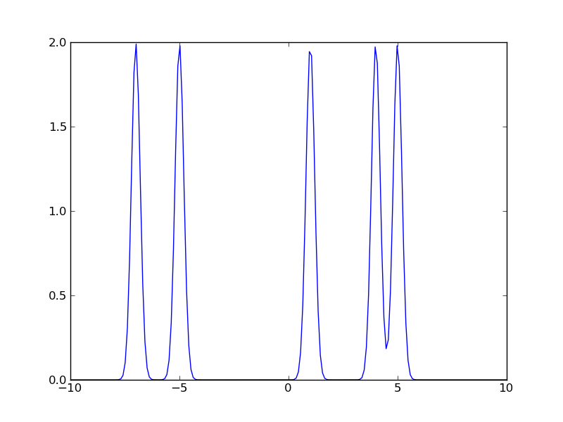
>>> data = np.array([-7.0, -5.0, 1.0, 4.0, 5.0])
Plot the sum of 5 gaussians with the mean equal to the data points specified above, and a standard deviation of 0.2. Plot in the range [-10, +10].
Solution:
>>> x = np.linspace(-10., +10, 200)
>>> y = np.zeros_like(x)
>>> for value in data:
...     y = y + stats.norm.pdf(x, loc=value, scale=0.2)
>>> plt.plot(x,y)
Now repeat the exercise for a standard deviation of 1.0, and a standard deviation of 3.0. In the context of kernel density estimates, the standard deviation is called the “bandwidth”. Choosing the bandwidth for a kernel corresponds to choosing the bin width for a histogram.
Let’s turn to a more realistic dataset:
>>> data = stats.norm.rvs(loc = 2.0, scale = 0.4, size = 200)
>>> mydensity = stats.gaussian_kde(data)
>>> x = np.linspace(0.0, 4.0, 200)
>>> y = mydensity(x)
>>> plt.plot(x,y)
>>> plt.scatter(data, zeros_like(data), marker='+')
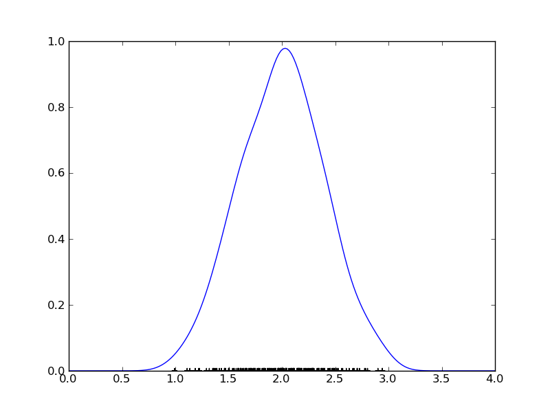
How does scipy choose the proper bandwidth? It has a few build-in rules-of-thumb. The standard one is Scott’s rule: n**(-1./(d+4)) with n the number of data points and d the number of dimenions (1 in our case). Another possibility is to use Silverman’s rule: n * (d + 2) / 4.)**(-1. / (d + 4)). See the manual for more information.
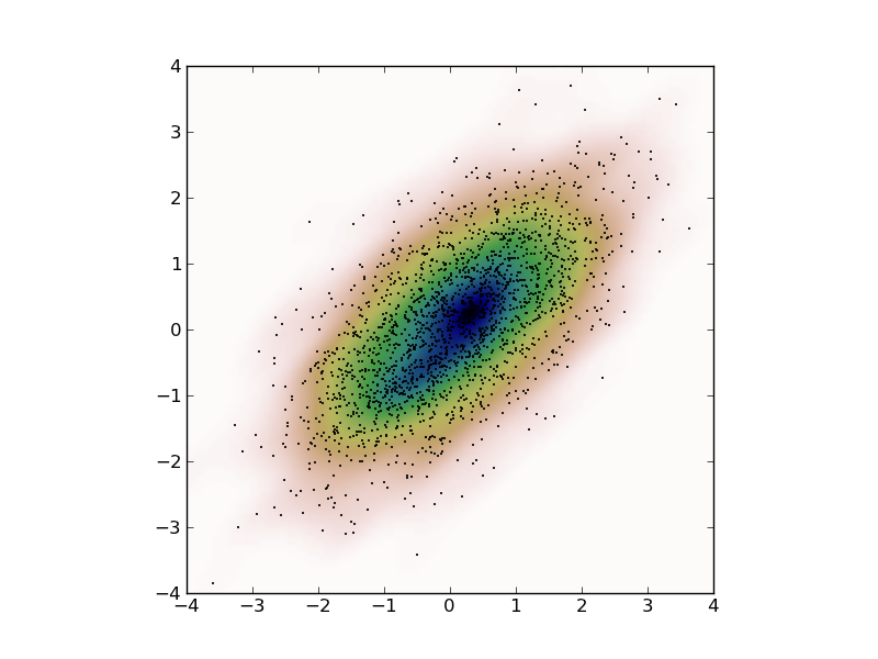
Kernel density estimates can also be done in 2 (or a higher number of) dimensions. Here is an example. First some artificial data:
>>> x = stats.norm.rvs(size=2000)
>>> y = stats.norm.rvs(scale=0.5, size=2000)
>>> data = np.vstack([x+y, x-y])
So, we just created some 2D correlated gaussian data. Now we compute the kernel density:
>>> mydensity = stats.gaussian_kde(data)
which we evaluate in a dense rectangular grid to plot:
>>> X, Y = np.mgrid[-4:4:100j, -4:4:100j]
>>> grid = np.vstack([X.ravel(), Y.ravel()])
>>> Z = mydensity(grid)
>>> Z = np.reshape(Z, X.shape)
Now we are ready to plot everything
>>> plt.imshow(np.rot90(Z), cmap=plt.cm.gist_earth, extent=[-4,+4,-4,+4])
>>> plt.plot(data[0], data[1], 'k.', markersize=2)
>>> plt.xlim([-4,+4])
>>> plt.ylim([-4,+4])